Last updated: 2025/06/06
XRAIN偏波レーダの生データから反射率や粒子判別結果のCAPPIデータを作成する方法はXRAIN偏波レーダによる降水粒子判別に説明しました。このページは作成されたCAPPIデータの解析方法を説明します。
データを読み込むにはPythonモジュールnetCDF4が必要です。インストールの方法はPythonの環境によるので、各自調べてください。
# SSHサーバには必要なモジュールがすべてインストールされているので、直接SSHサーバ上で図を作成することもできます。ただ、以下の3のXRAIN_viewer.pyの使用はSSHサーバ上はできません。
1. CAPPI (一定高度の平面図)の作成
以下のコードでCAPPIの図を作成できます。以下の3つのパラメータを設定する必要があります。
- 行9の
plotTypeはデータの種類を指定する。1は反射率、2は粒子の種類です。 - 行10の
plotHeightはプロットする平面の高度です。単位はkmで、0.25から16までの数値に指定してください。 - 行11の
fileNameは作成されたCAPPIデータの一つのフールパスです。
また、背景に境界線地図をプロットする場合は行47〜49をコメント解除し、行47に地図のデータのフールパスを指定してください。(https://tingwu.info/pylab/lab03.html に参照)
#!/usr/bin/env python3

import numpy as np
import datetime
import netCDF4
import matplotlib.pyplot as plt
import matplotlib.cm as cm

plotType = 2 # 1: reflectivity; 2: precipitation type
plotHeight = 1.25 #km; 0.25<=plotHeight<=16 km with 0.25 km resolution
fileName = '/media/DISK/XRAIN_CAPPI/20211101/NOU/CAPPI202111012020.nc'

#Other than 'REF' and 'HCX', strType can also be 'ZDR', 'KDP' and 'RHOHV', but code for plotting should be added after line 61
if plotType==1:
    strType = 'REF'
elif plotType==2:
    strType = 'HCX'
else:
    raise SystemExit('Data type not recognized: '+str(plotType))
if plotHeight<0.25 or plotHeight>16:
    raise SystemExit('Invalid height value: '+str(plotHeight))

f = netCDF4.Dataset(fileName)
lat, lon = f.variables['LAT'], f.variables['LON']

radarTime = f.variables['TIME'][:]
strNatTime = datetime.datetime.fromtimestamp(int(radarTime)).strftime('%Y%m%d-%H:%M:%S')
print(strNatTime)

heightIndex = int(round((plotHeight-0.25)/0.25))
dataMat = f.variables[strType][0,heightIndex,:,:]

le = 0.10
re = 0.07
w2 = 0.04
hb = 0.03
w1 = 1-le-re-w2-hb

te = 0.06
be = 0.09
h = 1-te-be

f = plt.figure(figsize=(8, 7))
ax1 = f.add_axes([le, be, w1, h])
ax2 = f.add_axes([le+w1+hb, be, w2, h])

# mapData = '/home/username/japanmap.npy'
# mapMat = np.load(mapData)
# ax1.plot(mapMat[:, 0], mapMat[:, 1], c='k', lw=0.5)

if plotType==1:
    c = ax1.contourf(lon[:], lat[:], dataMat, levels = np.arange(5, 55, 1), cmap='jet')
    cb = plt.colorbar(c, cax = ax2)
    ax2.text(0.5, 1.005, 'dBZ', ha='center', va='bottom', fontsize=14, transform = ax2.transAxes)
elif plotType==2:
    my_cmap = cm.get_cmap('jet', 8)
    my_cmap.set_under(alpha=0)
    c = ax1.pcolormesh(lon[:], lat[:], dataMat, cmap=my_cmap, vmin=1, vmax=9)
    cb = plt.colorbar(c, ticks=np.arange(1.5, 9, 1), cax = ax2)
    cb.ax.set_yticklabels([str(i) for i in range(1,9)])
    ax2.text(0.5, 1.005, 'Type', ha='center', va='bottom', fontsize=14, transform = ax2.transAxes)

ax1.set_xlim([135.6, 137.5])
ax1.set_ylim([35.6, 37.3])
ax1.set_xlabel('Longitude (Degree E)')
ax1.set_ylabel('Latitude (Degree N)')
ax1.set_title(strNatTime+' (JST) '+str(plotHeight)+' km')
plt.savefig('/home/username/CAPPI_'+fileName[-15:-4]+'.png', dpi=300)
#plt.show()
#!/usr/bin/env python3
import numpy as np
import datetime
import netCDF4
import matplotlib.pyplot as plt
import matplotlib.cm as cm
plotType = 2 # 1: reflectivity; 2: precipitation type
plotHeight = 1.25 #km; 0.25<=plotHeight<=16 km with 0.25 km resolution
fileName = '/media/DISK/XRAIN_CAPPI/20211101/NOU/CAPPI202111012020.nc'
#Other than 'REF' and 'HCX', strType can also be 'ZDR', 'KDP' and 'RHOHV', but code for plotting should be added after line 61
if plotType==1:
strType = 'REF'
elif plotType==2:
strType = 'HCX'
else:
raise SystemExit('Data type not recognized: '+str(plotType))
if plotHeight<0.25 or plotHeight>16:
raise SystemExit('Invalid height value: '+str(plotHeight))
f = netCDF4.Dataset(fileName)
lat, lon = f.variables['LAT'], f.variables['LON']
radarTime = f.variables['TIME'][:]
strNatTime = datetime.datetime.fromtimestamp(int(radarTime)).strftime('%Y%m%d-%H:%M:%S')
print(strNatTime)
heightIndex = int(round((plotHeight-0.25)/0.25))
dataMat = f.variables[strType][0,heightIndex,:,:]
le = 0.10
re = 0.07
w2 = 0.04
hb = 0.03
w1 = 1-le-re-w2-hb
te = 0.06
be = 0.09
h = 1-te-be
f = plt.figure(figsize=(8, 7))
ax1 = f.add_axes([le, be, w1, h])
ax2 = f.add_axes([le+w1+hb, be, w2, h])
# mapData = '/home/username/japanmap.npy'
# mapMat = np.load(mapData)
# ax1.plot(mapMat[:, 0], mapMat[:, 1], c='k', lw=0.5)
if plotType==1:
c = ax1.contourf(lon[:], lat[:], dataMat, levels = np.arange(5, 55, 1), cmap='jet')
cb = plt.colorbar(c, cax = ax2)
ax2.text(0.5, 1.005, 'dBZ', ha='center', va='bottom', fontsize=14, transform = ax2.transAxes)
elif plotType==2:
my_cmap = cm.get_cmap('jet', 8)
my_cmap.set_under(alpha=0)
c = ax1.pcolormesh(lon[:], lat[:], dataMat, cmap=my_cmap, vmin=1, vmax=9)
cb = plt.colorbar(c, ticks=np.arange(1.5, 9, 1), cax = ax2)
cb.ax.set_yticklabels([str(i) for i in range(1,9)])
ax2.text(0.5, 1.005, 'Type', ha='center', va='bottom', fontsize=14, transform = ax2.transAxes)
ax1.set_xlim([135.6, 137.5])
ax1.set_ylim([35.6, 37.3])
ax1.set_xlabel('Longitude (Degree E)')
ax1.set_ylabel('Latitude (Degree N)')
ax1.set_title(strNatTime+' (JST) '+str(plotHeight)+' km')
plt.savefig('/home/username/CAPPI_'+fileName[-15:-4]+'.png', dpi=300)
#plt.show()*strTypeをZDR, KDP, RHOHVに設定することもできるが、図をプロットする部分のコードを修正する必要があります。
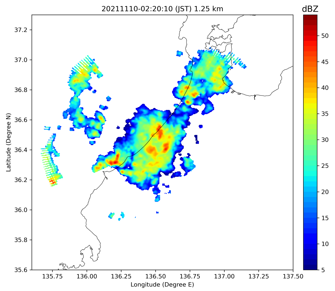
作成した反射率の図は以下のようになります。
作成した粒子判定結果の図は以下のようになります。
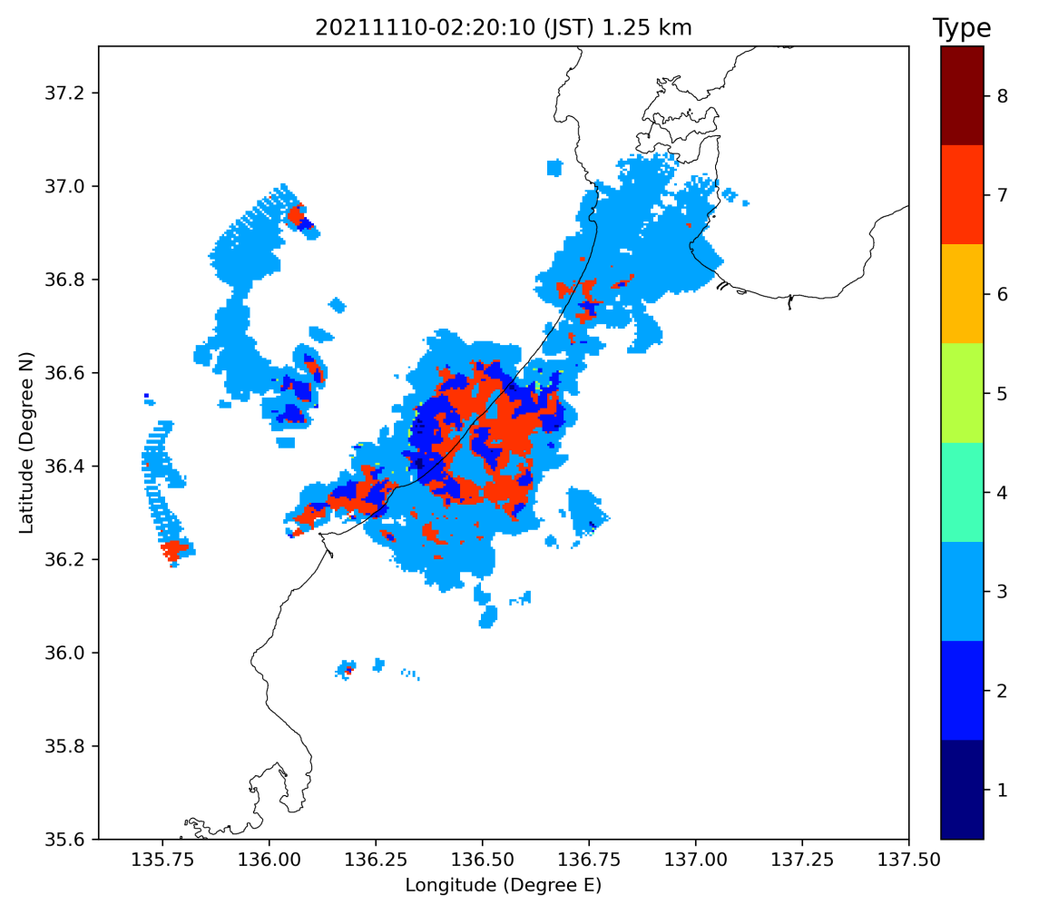
粒子判別結果の数値
1: 霧雨(ドリズル)
2: 雨
3: 湿雪(融けかけの雪片)
4: 乾雪(雪片)
5: 氷晶
6: 乾霰
7: 湿霰(融けかけの霰)
8: 雨+雹
RHI (断面図)の作成
以下のコードでRHIの図を作成できます。以下のパラメータを設定する必要があります。
- 行9〜12: 断面を切る直線の開始点と終了点の緯度経度
- 行14の
plotTypeはデータの種類を指定する。1は反射率、2は粒子の種類です。 - 行15の
maxHeightは表示する最大の高さです。 - 行16の
fileNameは作成されたCAPPIデータの一つのフールパスです。
#!/usr/bin/env python3

import netCDF4
import numpy as np
import datetime
import matplotlib.pyplot as plt
import matplotlib.cm as cm

lati1 = 36.4
longi1 = 135.75
lati2 = 36.6
longi2 = 136.25

plotType = 1 # 1 for reflectivity; 2 for precipitation type
maxHeight = 8 #km
fileName = '/media/DISK/XRAIN_CAPPI/20211110/NOU/CAPPI202111100400.nc'

if plotType==1:
    strType = 'REF'
elif plotType==2:
    strType = 'HCX'
else:
    raise SystemExit('Data type not recognized: '+str(plotType))

R = 6370.519
def dis(lati1, longi1, lati2, longi2):
    lati1 = lati1/180*np.pi
    longi1 = longi1/180*np.pi
    lati2 = lati2/180*np.pi
    longi2 = longi2/180*np.pi
    return R*np.arccos(np.sin(lati1)*np.sin(lati2)+np.cos(lati1)*np.cos(lati2)*np.cos(longi1-longi2))
disVal = dis(lati1, longi1, lati2, longi2)

f = netCDF4.Dataset(fileName)
lat, lon = f.variables['LAT'], f.variables['LON']
radarTime = f.variables['TIME'][:]
strNatTime = datetime.datetime.fromtimestamp(int(radarTime)).strftime('%Y%m%d-%H:%M:%S')
print(strNatTime)

latiLen = len(lat)
latiResi = (lat[-1]-lat[0])/(latiLen-1)
longiLen = len(lon)
longiResi = (lon[-1]-lon[0])/(longiLen-1)
x1 = (longi1-lon[0])/longiResi
y1 = (lati1-lat[0])/latiResi
x2 = (longi2-lon[0])/longiResi
y2 = (lati2-lat[0])/latiResi
xDiffer = abs(x1-x2)
yDiffer = abs(y1-y2)

#Contruct points along the line
xIndex1 = int(x1)
yIndex1 = int(y1)
xIndex2 = int(x2)
yIndex2 = int(y2)
if xDiffer>yDiffer: #Determine X, calculate Y at each value of X
    if x1>x2:
        xPointMat = np.arange(xIndex1, xIndex2-1, -1)
    else:
        xPointMat = np.arange(xIndex1, xIndex2+1)
    yPointMat = np.zeros(len(xPointMat), dtype=int)
    for i in range(len(xPointMat)):
        xPointVal = xPointMat[i]
        yPointVal = float(x1*y2-x2*y1+xPointVal*y1-xPointVal*y2)/(x1-x2)
        yPointMat[i] = int(round(yPointVal))
else:#Determine Y, calculate X at each value of Y
    if y1>y2:
        yPointMat = np.arange(yIndex1, yIndex2-1, -1)
    else:
        yPointMat = np.arange(yIndex1, yIndex2+1)
    xPointMat = np.zeros(len(yPointMat), dtype=int)
    for i in range(len(yPointMat)):
        yPointVal = yPointMat[i]
        xPointVal = float(x1*yPointVal-x2*yPointVal+x2*y1-x1*y2)/(y1-y2)
        xPointMat[i] = int(round(xPointVal))

#Get data
plotDataMat = []
layerNum = int(maxHeight/0.25)+1
for i in range(layerNum):
    layerMat = f.variables[strType][0,i,:,:]
    for j in range(len(xPointMat)):
        plotDataMat.append(layerMat[yPointMat[j], xPointMat[j]])
plotDataMat = np.reshape(plotDataMat, (layerNum, len(xPointMat)))

#Plot
le = 0.06
re = 0.04
w2 = 0.03
hb = 0.02
w1 = 1-le-re-w2-hb
te = 0.07
be = 0.12
h = 1-te-be
f = plt.figure(figsize=(9, 4))
ax1 = f.add_axes([le, be, w1, h])
ax2 = f.add_axes([le+w1+hb, be, w2, h])

xMat = np.linspace(0, disVal, len(xPointMat), endpoint=True)
yMat = np.arange(0.25, layerNum*0.25+0.1, 0.25)
if plotType==1:
    c = ax1.contourf(xMat, yMat, plotDataMat, levels = np.arange(5, 55, 1), cmap='jet')
    cb = plt.colorbar(c, cax = ax2)
    ax2.text(0.5, 1.005, 'dBZ', ha='center', va='bottom', fontsize=14, transform = ax2.transAxes)
elif plotType==2:
    my_cmap = cm.get_cmap('jet', 8)
    my_cmap.set_under(alpha=0)
    c = ax1.pcolormesh(xMat, yMat, plotDataMat, cmap=my_cmap, vmin=1, vmax=9)
    cb = plt.colorbar(c, ticks=np.arange(1.5, 9, 1), cax = ax2)
    cb.ax.set_yticklabels([str(i) for i in range(1,9)])
    ax2.text(0.5, 1.005, 'Type', ha='center', va='bottom', fontsize=14, transform = ax2.transAxes)

ax1.set_xlim([0, disVal])
ax1.set_ylim([0, layerNum*0.25])
ax1.set_xlabel('Distance (km)')
ax1.set_ylabel('Height (km)')
ax1.set_title(strNatTime+' (JST) ')
plt.savefig('/home/username/RHI_'+fileName[-15:-4]+'.png', dpi=300)
# plt.show()
#!/usr/bin/env python3
import netCDF4
import numpy as np
import datetime
import matplotlib.pyplot as plt
import matplotlib.cm as cm
lati1 = 36.4
longi1 = 135.75
lati2 = 36.6
longi2 = 136.25
plotType = 1 # 1 for reflectivity; 2 for precipitation type
maxHeight = 8 #km
fileName = '/media/DISK/XRAIN_CAPPI/20211110/NOU/CAPPI202111100400.nc'
if plotType==1:
strType = 'REF'
elif plotType==2:
strType = 'HCX'
else:
raise SystemExit('Data type not recognized: '+str(plotType))
R = 6370.519
def dis(lati1, longi1, lati2, longi2):
lati1 = lati1/180*np.pi
longi1 = longi1/180*np.pi
lati2 = lati2/180*np.pi
longi2 = longi2/180*np.pi
return R*np.arccos(np.sin(lati1)*np.sin(lati2)+np.cos(lati1)*np.cos(lati2)*np.cos(longi1-longi2))
disVal = dis(lati1, longi1, lati2, longi2)
f = netCDF4.Dataset(fileName)
lat, lon = f.variables['LAT'], f.variables['LON']
radarTime = f.variables['TIME'][:]
strNatTime = datetime.datetime.fromtimestamp(int(radarTime)).strftime('%Y%m%d-%H:%M:%S')
print(strNatTime)
latiLen = len(lat)
latiResi = (lat[-1]-lat[0])/(latiLen-1)
longiLen = len(lon)
longiResi = (lon[-1]-lon[0])/(longiLen-1)
x1 = (longi1-lon[0])/longiResi
y1 = (lati1-lat[0])/latiResi
x2 = (longi2-lon[0])/longiResi
y2 = (lati2-lat[0])/latiResi
xDiffer = abs(x1-x2)
yDiffer = abs(y1-y2)
#Contruct points along the line
xIndex1 = int(x1)
yIndex1 = int(y1)
xIndex2 = int(x2)
yIndex2 = int(y2)
if xDiffer>yDiffer: #Determine X, calculate Y at each value of X
if x1>x2:
xPointMat = np.arange(xIndex1, xIndex2-1, -1)
else:
xPointMat = np.arange(xIndex1, xIndex2+1)
yPointMat = np.zeros(len(xPointMat), dtype=int)
for i in range(len(xPointMat)):
xPointVal = xPointMat[i]
yPointVal = float(x1*y2-x2*y1+xPointVal*y1-xPointVal*y2)/(x1-x2)
yPointMat[i] = int(round(yPointVal))
else:#Determine Y, calculate X at each value of Y
if y1>y2:
yPointMat = np.arange(yIndex1, yIndex2-1, -1)
else:
yPointMat = np.arange(yIndex1, yIndex2+1)
xPointMat = np.zeros(len(yPointMat), dtype=int)
for i in range(len(yPointMat)):
yPointVal = yPointMat[i]
xPointVal = float(x1*yPointVal-x2*yPointVal+x2*y1-x1*y2)/(y1-y2)
xPointMat[i] = int(round(xPointVal))
#Get data
plotDataMat = []
layerNum = int(maxHeight/0.25)+1
for i in range(layerNum):
layerMat = f.variables[strType][0,i,:,:]
for j in range(len(xPointMat)):
plotDataMat.append(layerMat[yPointMat[j], xPointMat[j]])
plotDataMat = np.reshape(plotDataMat, (layerNum, len(xPointMat)))
#Plot
le = 0.06
re = 0.04
w2 = 0.03
hb = 0.02
w1 = 1-le-re-w2-hb
te = 0.07
be = 0.12
h = 1-te-be
f = plt.figure(figsize=(9, 4))
ax1 = f.add_axes([le, be, w1, h])
ax2 = f.add_axes([le+w1+hb, be, w2, h])
xMat = np.linspace(0, disVal, len(xPointMat), endpoint=True)
yMat = np.arange(0.25, layerNum*0.25+0.1, 0.25)
if plotType==1:
c = ax1.contourf(xMat, yMat, plotDataMat, levels = np.arange(5, 55, 1), cmap='jet')
cb = plt.colorbar(c, cax = ax2)
ax2.text(0.5, 1.005, 'dBZ', ha='center', va='bottom', fontsize=14, transform = ax2.transAxes)
elif plotType==2:
my_cmap = cm.get_cmap('jet', 8)
my_cmap.set_under(alpha=0)
c = ax1.pcolormesh(xMat, yMat, plotDataMat, cmap=my_cmap, vmin=1, vmax=9)
cb = plt.colorbar(c, ticks=np.arange(1.5, 9, 1), cax = ax2)
cb.ax.set_yticklabels([str(i) for i in range(1,9)])
ax2.text(0.5, 1.005, 'Type', ha='center', va='bottom', fontsize=14, transform = ax2.transAxes)
ax1.set_xlim([0, disVal])
ax1.set_ylim([0, layerNum*0.25])
ax1.set_xlabel('Distance (km)')
ax1.set_ylabel('Height (km)')
ax1.set_title(strNatTime+' (JST) ')
plt.savefig('/home/username/RHI_'+fileName[-15:-4]+'.png', dpi=300)
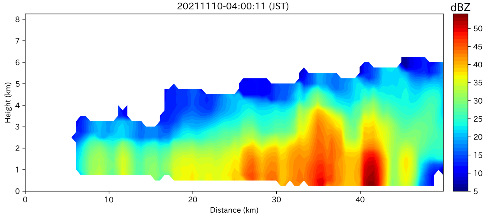
# plt.show()作成した反射率のRHIは以下のようになります。
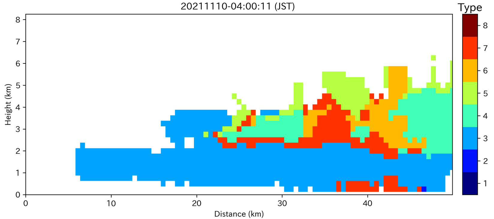
作成した粒子判定結果のRHIは以下のようになります。
3. 解析プログラム XRAIN_viewer.py
以下のプログラムXRAIN_viewer.pyを利用すれば、キーボードやマウスの操作でデータ表示の切り替え等が簡単にできます。
XRAIN_viewer.py
パラメータの設定
- 行11の
startFileは最初に表示するデータファイルのフールパスです。同じフォルダーにあるデータは下記の通りキーボードの操作で表示することができます。 - 行12の
plotTypeはデータの種類を指定する。1は反射率、2は粒子の種類です。
操作方法
aキー: 同じフォルダーにある一つ前の時刻のデータを表示するdキー: 同じフォルダーにある次の時刻のデータを表示する- \uparrow: 一つ上の高度の平面図を表示する
- \downarrow: 一つ下の高度の平面図を表示する
tキー: マウスのところの緯度経度、反射率あるいは粒子種類の数値をプリントする- マウスをドラッグすることで拡大することができる
- \leftarrow: その前に表示した範囲に戻る
- \rightarrow: その逆
qキー:qを押すと、コマンドプロンプトにCurrent function: plot RHIがプリントされる。この状態でマウスをドラッグすると、マウスが書いた直線にある断面図が表示される。qをもう一回押すと、Current function: enlarge an areaが表示され、拡大機能に戻る。1と2キー: 雷雲移動速度の計算。1キーで開始点を選んで、2キーで(別の時刻)の終了点を選んだら、X方向とY方向の移動速度がプリントされる。
このプログラムの上にさまざまな機能を加えることができます。自分の解析目的に合わせて、いろいろいじってみてください。
Back to Python関連資料