Classification of radiation waveforms of positive and negative return strokes

Last updated: 2023/07/23

This page describes a simple Python script to use the classifiers built in the paper "High-Accuracy Classification of Radiation Waveforms of Lightning Return Strokes" published in JGR Atmosphere (https://doi.org/10.1029/2023JD038715)

1. Download the data of the trained models

Data of the trained models can be found at the following page:
https://doi.org/10.5281/zenodo.7900171 (model.zip)
NRS.pkl and NRS_statis.npy are necessary for using the classifier for negative return strokes.
PRS.pkl and PRS_statis.npy are necessary for using the classifier for positive return strokes.

2. FALMA waveform data sample

One FALMA waveform data file for demonstrating the usage of the classifiers can be found at the following page:
https://doi.org/10.5281/zenodo.7900171 (script.zip => GFUL1659592956.bz2)
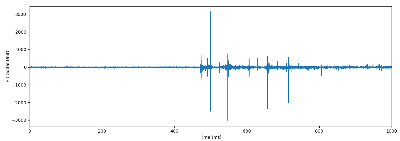
It contains one-second waveform data recorded at 2022/08/04 15:02:36 (JST). The sampling rate is 1 MS/s. It contains at least 2 -RSs and 3 +RSs. These RSs are around 200 km from the recording site. The waveform is recorded using the atmospheric electricity sign convention, so a -RS produces a positive pulse. Details of FALMA waveform data can be found at the following page:
https://tingwu.info/pylab/lab05.html

The following figure shows the 1-sec waveform.

3. Simplifications and limitations

In order to make the Python script as easy to understand as possible, some simplifications are made here.

Only the data of one site is used here. In order to achieve high accuracy and efficiency, it is important to use data of multiple sites (preferably >4) and for every parameter calculate the median value.
A fixed trigger level is used here and the largest positive and negative pulses in every window, if larger than the trigger level, are classified. In practice, it is necessary to first locate every pulse, and for every located pulse, use waveforms recorded at appropriate distances (larger than 40 km and within a few hundred km) to calculate the parameters.
Some other simplifications are written as comments in the script.

There are also some limitations of the classifiers.

The classifier for -RSs is trained using a compact FALMA network, so it may not have equally high performance when used in a large network. It is expected that the accuracy and efficiency decrease with increasing distances. You may also try the classifier for remote negative RSs in section 4.
The classifier for -RSs may not work well for winter lightning, as it is known that -RSs in winter, especially the strong ones, usually produce special waveforms (Wu et al., 2021, JGR; Wu et al., 2021, GRL).
Large local noises are expected to have some influences, as we believe our sites are mostly at locations with relatively low noises.

3. Python script

In order to run the script, it is necessary to first change the full path of the waveform data at line 20 and the directory storing the trained models at line 42.

#!/usr/bin/env python3

'''
This is a simple script to show how to use the classifiers reported in the paper:
    High-Accuracy Classification of Radiation Waveforms of Lightning Return Strokes (JGR Atmosphere, 2023)
Detailed descriptions and possible future updates of the classifiers can be found in the following page:
    https://tingwu.info/pylab/classifier.html
For more information, please contact:
    Ting Wu (wu.ting.x4@f.gifu-u.ac.jp)
'''

import numpy as np
import bz2
import joblib
from os.path import join

#Read one FALMA data file
#Format of FALMA waveform data is described in the following page:
#https://tingwu.info/pylab/lab05.html
fidData = bz2.BZ2File('GFUL1659592956.bz2')#Change it to the full path of the data file
dataMat = np.frombuffer(fidData.read(), np.int16)
fidData.close()

probaThre = 50 #%, pulses with probability higher than this value are treated as RSs

trigLev = 200 #Positive pulses with peaks larger than trigLev and negative pulses with peaks smaller than -trigLev will be classified
              #For simplicity, a fixed trigLev is used here

sampRate = 1000 #samples per ms
dataTimeLen = 1000 #ms, recording length of one data file
windowTimeLen = 20 #ms, window length. No more than one positive and one negative pulses are examined in one window
                    #Smaller window lengths such as 10 ms are also fine

windowLen = windowTimeLen*sampRate #window length in data points
dataLen = dataTimeLen*sampRate #Number of data points in one data file
windowNum = int(round(dataLen/windowLen)) #Number of windows in one data file
pulseLeftLen = int(round(0.3*sampRate)) #Data points needed to form a pulse, 300 us left of the peak
pulseRightLen = int(round(0.4*sampRate)) #400 us right of the peak
pulseLen = pulseLeftLen+pulseRightLen

#Data of the trained classifiers
modelDir = 'model'#Change it to the full path
modelN = joblib.load(join(modelDir, 'NRS.pkl'))
[sN, mN] = np.load(join(modelDir, 'NRS_statis.npy'))
modelP = joblib.load(join(modelDir, 'PRS.pkl'))
[sP, mP] = np.load(join(modelDir, 'PRS_statis.npy'))


#The function for calculating pulse parameters
def calParaFun(pulseMat):
    peakIndex = pulseLeftLen
    peakAmp = pulseMat[peakIndex]
    
    #Calculate rise time, fall time, half peak time
    #50% peak before the peak
    tarAmp = peakAmp*0.5
    curIndex = peakIndex
    while pulseMat[curIndex]>tarAmp and curIndex>0:
        curIndex -= 1
    if pulseMat[curIndex+1]==pulseMat[curIndex]:
        halfBefIndex = curIndex+0.5
    else:#Linear interpolation
        halfBefIndex = (tarAmp-pulseMat[curIndex])/(pulseMat[curIndex+1]-pulseMat[curIndex])+curIndex
    
    #10% peak
    tarAmp = peakAmp*0.1
    while pulseMat[curIndex]>tarAmp and curIndex>0:
        curIndex -= 1
    if pulseMat[curIndex+1]==pulseMat[curIndex]:
        tenPerIndex = curIndex+0.5
    else:
        tenPerIndex = (tarAmp-pulseMat[curIndex])/(pulseMat[curIndex+1]-pulseMat[curIndex])+curIndex
    
    #50% peak after the peak
    tarAmp = peakAmp*0.5
    curIndex = peakIndex
    while pulseMat[curIndex]>tarAmp and curIndex<pulseLen-1:
        curIndex += 1
    if pulseMat[curIndex-1]==pulseMat[curIndex]:
        halfAftIndex = curIndex-0.5
    else:
        halfAftIndex = curIndex-(tarAmp-pulseMat[curIndex])/(pulseMat[curIndex-1]-pulseMat[curIndex])
    
    #zero crossing after the peak
    tarAmp = 0
    while pulseMat[curIndex]>tarAmp and curIndex<pulseLen-1:
        curIndex += 1
    if pulseMat[curIndex-1]==pulseMat[curIndex]:
        zeroIndex = curIndex-0.5
    else:
        zeroIndex = curIndex-(tarAmp-pulseMat[curIndex])/(pulseMat[curIndex-1]-pulseMat[curIndex])
    
    T_rise = (peakIndex-tenPerIndex)/sampRate*1000
    T_fall = (zeroIndex-peakIndex)/sampRate*1000
    T_half = (halfAftIndex-halfBefIndex)/sampRate*1000
    
    #Calculate ratios
    if T_rise<50:#us, In case the rise time is abnormally long
        index1 = int(round(tenPerIndex))
    else:
        index1 = int(peakIndex-50/1000*sampRate)
    indexBef = peakIndex-int(round(0.1*sampRate))
    befPAmpNear = max(pulseMat[indexBef:index1])
    befNAmpNear = min(pulseMat[indexBef:index1])
    befPAmpFar = max(pulseMat[0:indexBef])
    befNAmpFar = min(pulseMat[0:indexBef])
    
    if T_fall<100:#us, in case the fall time is abnormally long
        index2 = int(round(zeroIndex))
    else:
        index2 = int(peakIndex+100/1000*sampRate)
    indexAft = peakIndex+int(round(0.2*sampRate))
    aftPAmpNear = max(pulseMat[index2:indexAft])
    aftNAmpNear = min(pulseMat[index2:indexAft])
    aftPAmpFar = max(pulseMat[indexAft:])
    aftNAmpFar = min(pulseMat[indexAft:])
    
    #The denominators should not be zero 
    #If any of the denominators is zero, normally it indicates the data has some problem
    #In practice, some special treatment should be made for zero denominators
    R_bp1 = peakAmp/befPAmpNear
    R_bn1 = peakAmp/befNAmpNear
    R_bp2 = peakAmp/befPAmpFar
    R_bn2 = peakAmp/befNAmpFar
    R_ap1 = peakAmp/aftPAmpNear
    R_an1 = peakAmp/aftNAmpNear
    R_ap2 = peakAmp/aftPAmpFar
    R_an2 = peakAmp/aftNAmpFar
    
    return [T_rise, T_fall, T_half, R_bp1, R_bn1, R_bp2, R_bn2, R_ap1, R_an1, R_ap2, R_an2]


for polaIndex in [1, -1]: # 1 for classify -RS, -1 for classify +RS (waveforms are in atmospheric electricity sign convention)
    dataMatPola = dataMat*polaIndex 
    for i in range(windowNum):   
        windowData = dataMatPola[i*windowLen:(i+1)*windowLen]
        peakIndex = np.argmax(windowData)+i*windowLen
        if peakIndex<pulseLeftLen or peakIndex+pulseRightLen>dataLen:#A simple treatment for peaks at the beginning and the end
            continue                                                 #In practice, they should also be carefully examined
            
        peakAmp = dataMatPola[peakIndex]
        if peakAmp>trigLev:
            #Get data points needed for a pulse and pass the data to calParaFun
            pulseData = dataMatPola[peakIndex-pulseLeftLen:peakIndex+pulseRightLen]
            paraMat = calParaFun(pulseData)

            if polaIndex>0:#Trained data of -RS
                testModel = modelN
                m = mN
                s = sN
            else:#Trained data of +RS
                testModel = modelP
                m = mP
                s = sP
            paraMat = np.array([paraMat]-m)/s
            probaVal = testModel.predict_proba(paraMat)
            probaVal = probaVal[0][1]*100 #Probability that the pulse is an RS
            if probaVal<probaThre:
                continue
            
            if polaIndex>0:
                print('-RS (probability:%3d, peak time: %7.3f ms)' % (probaVal, peakIndex/sampRate))
            else:
                print('+RS (probability:%3d, peak time: %7.3f ms)' % (probaVal, peakIndex/sampRate))

#!/usr/bin/env python3

'''
This is a simple script to show how to use the classifiers reported in the paper:
    High-Accuracy Classification of Radiation Waveforms of Lightning Return Strokes (JGR Atmosphere, 2023)
Detailed descriptions and possible future updates of the classifiers can be found in the following page:
    https://tingwu.info/pylab/classifier.html
For more information, please contact:
    Ting Wu (wu.ting.x4@f.gifu-u.ac.jp)
'''

import numpy as np
import bz2
import joblib
from os.path import join

#Read one FALMA data file
#Format of FALMA waveform data is described in the following page:
#https://tingwu.info/pylab/lab05.html
fidData = bz2.BZ2File('GFUL1659592956.bz2')#Change it to the full path of the data file
dataMat = np.frombuffer(fidData.read(), np.int16)
fidData.close()

probaThre = 50 #%, pulses with probability higher than this value are treated as RSs

trigLev = 200 #Positive pulses with peaks larger than trigLev and negative pulses with peaks smaller than -trigLev will be classified
              #For simplicity, a fixed trigLev is used here

sampRate = 1000 #samples per ms
dataTimeLen = 1000 #ms, recording length of one data file
windowTimeLen = 20 #ms, window length. No more than one positive and one negative pulses are examined in one window
                    #Smaller window lengths such as 10 ms are also fine

windowLen = windowTimeLen*sampRate #window length in data points
dataLen = dataTimeLen*sampRate #Number of data points in one data file
windowNum = int(round(dataLen/windowLen)) #Number of windows in one data file
pulseLeftLen = int(round(0.3*sampRate)) #Data points needed to form a pulse, 300 us left of the peak
pulseRightLen = int(round(0.4*sampRate)) #400 us right of the peak
pulseLen = pulseLeftLen+pulseRightLen

#Data of the trained classifiers
modelDir = 'model'#Change it to the full path
modelN = joblib.load(join(modelDir, 'NRS.pkl'))
[sN, mN] = np.load(join(modelDir, 'NRS_statis.npy'))
modelP = joblib.load(join(modelDir, 'PRS.pkl'))
[sP, mP] = np.load(join(modelDir, 'PRS_statis.npy'))


#The function for calculating pulse parameters
def calParaFun(pulseMat):
    peakIndex = pulseLeftLen
    peakAmp = pulseMat[peakIndex]
    
    #Calculate rise time, fall time, half peak time
    #50% peak before the peak
    tarAmp = peakAmp*0.5
    curIndex = peakIndex
    while pulseMat[curIndex]>tarAmp and curIndex>0:
        curIndex -= 1
    if pulseMat[curIndex+1]==pulseMat[curIndex]:
        halfBefIndex = curIndex+0.5
    else:#Linear interpolation
        halfBefIndex = (tarAmp-pulseMat[curIndex])/(pulseMat[curIndex+1]-pulseMat[curIndex])+curIndex
    
    #10% peak
    tarAmp = peakAmp*0.1
    while pulseMat[curIndex]>tarAmp and curIndex>0:
        curIndex -= 1
    if pulseMat[curIndex+1]==pulseMat[curIndex]:
        tenPerIndex = curIndex+0.5
    else:
        tenPerIndex = (tarAmp-pulseMat[curIndex])/(pulseMat[curIndex+1]-pulseMat[curIndex])+curIndex
    
    #50% peak after the peak
    tarAmp = peakAmp*0.5
    curIndex = peakIndex
    while pulseMat[curIndex]>tarAmp and curIndex<pulseLen-1:
        curIndex += 1
    if pulseMat[curIndex-1]==pulseMat[curIndex]:
        halfAftIndex = curIndex-0.5
    else:
        halfAftIndex = curIndex-(tarAmp-pulseMat[curIndex])/(pulseMat[curIndex-1]-pulseMat[curIndex])
    
    #zero crossing after the peak
    tarAmp = 0
    while pulseMat[curIndex]>tarAmp and curIndex<pulseLen-1:
        curIndex += 1
    if pulseMat[curIndex-1]==pulseMat[curIndex]:
        zeroIndex = curIndex-0.5
    else:
        zeroIndex = curIndex-(tarAmp-pulseMat[curIndex])/(pulseMat[curIndex-1]-pulseMat[curIndex])
    
    T_rise = (peakIndex-tenPerIndex)/sampRate*1000
    T_fall = (zeroIndex-peakIndex)/sampRate*1000
    T_half = (halfAftIndex-halfBefIndex)/sampRate*1000
    
    #Calculate ratios
    if T_rise<50:#us, In case the rise time is abnormally long
        index1 = int(round(tenPerIndex))
    else:
        index1 = int(peakIndex-50/1000*sampRate)
    indexBef = peakIndex-int(round(0.1*sampRate))
    befPAmpNear = max(pulseMat[indexBef:index1])
    befNAmpNear = min(pulseMat[indexBef:index1])
    befPAmpFar = max(pulseMat[0:indexBef])
    befNAmpFar = min(pulseMat[0:indexBef])
    
    if T_fall<100:#us, in case the fall time is abnormally long
        index2 = int(round(zeroIndex))
    else:
        index2 = int(peakIndex+100/1000*sampRate)
    indexAft = peakIndex+int(round(0.2*sampRate))
    aftPAmpNear = max(pulseMat[index2:indexAft])
    aftNAmpNear = min(pulseMat[index2:indexAft])
    aftPAmpFar = max(pulseMat[indexAft:])
    aftNAmpFar = min(pulseMat[indexAft:])
    
    #The denominators should not be zero 
    #If any of the denominators is zero, normally it indicates the data has some problem
    #In practice, some special treatment should be made for zero denominators
    R_bp1 = peakAmp/befPAmpNear
    R_bn1 = peakAmp/befNAmpNear
    R_bp2 = peakAmp/befPAmpFar
    R_bn2 = peakAmp/befNAmpFar
    R_ap1 = peakAmp/aftPAmpNear
    R_an1 = peakAmp/aftNAmpNear
    R_ap2 = peakAmp/aftPAmpFar
    R_an2 = peakAmp/aftNAmpFar
    
    return [T_rise, T_fall, T_half, R_bp1, R_bn1, R_bp2, R_bn2, R_ap1, R_an1, R_ap2, R_an2]


for polaIndex in [1, -1]: # 1 for classify -RS, -1 for classify +RS (waveforms are in atmospheric electricity sign convention)
    dataMatPola = dataMat*polaIndex 
    for i in range(windowNum):   
        windowData = dataMatPola[i*windowLen:(i+1)*windowLen]
        peakIndex = np.argmax(windowData)+i*windowLen
        if peakIndex<pulseLeftLen or peakIndex+pulseRightLen>dataLen:#A simple treatment for peaks at the beginning and the end
            continue                                                 #In practice, they should also be carefully examined
            
        peakAmp = dataMatPola[peakIndex]
        if peakAmp>trigLev:
            #Get data points needed for a pulse and pass the data to calParaFun
            pulseData = dataMatPola[peakIndex-pulseLeftLen:peakIndex+pulseRightLen]
            paraMat = calParaFun(pulseData)

            if polaIndex>0:#Trained data of -RS
                testModel = modelN
                m = mN
                s = sN
            else:#Trained data of +RS
                testModel = modelP
                m = mP
                s = sP
            paraMat = np.array([paraMat]-m)/s
            probaVal = testModel.predict_proba(paraMat)
            probaVal = probaVal[0][1]*100 #Probability that the pulse is an RS
            if probaVal<probaThre:
                continue
            
            if polaIndex>0:
                print('-RS (probability:%3d, peak time: %7.3f ms)' % (probaVal, peakIndex/sampRate))
            else:
                print('+RS (probability:%3d, peak time: %7.3f ms)' % (probaVal, peakIndex/sampRate))

Following is the output of the script:

-RS (probability: 50, peak time: 499.834 ms)
-RS (probability: 54, peak time: 628.981 ms)
+RS (probability: 98, peak time: 547.990 ms)
+RS (probability:100, peak time: 657.673 ms)
+RS (probability: 89, peak time: 715.490 ms)

We can see that two -RSs and three +RSs are identified. Note that the probability for the two -RSs are not very high, due to the fact that only the data of one site is used here. The large distance of these RSs may also have some influences.

If we decrease the probability threshold at line 24 to 30 (probaThre = 30), the result would be:

-RS (probability: 50, peak time: 499.834 ms)
-RS (probability: 46, peak time: 606.680 ms)
-RS (probability: 54, peak time: 628.981 ms)
-RS (probability: 30, peak time: 684.586 ms)
+RS (probability: 98, peak time: 547.990 ms)
+RS (probability:100, peak time: 657.673 ms)
+RS (probability: 89, peak time: 715.490 ms)

Two more pulses are identified as -RSs. If you check these two pulses carefully, you can see that they indeed share some similarities with -RSs, but it is somewhat difficult to determine whether they are truely -RSs.

4. Classifier for remote negative RSs

We also built a classifier for negative RSs with large distances (mainly between 100~300 km). If you are mainly observing lightning discharges in this range, you may try this classifier.

Download the following two files, use NRS_remote.pkl to replace NRS.pkl, and use NRS_remote_statis.npy to replace NRS_statis.npy in the script above.

NRS_remote.pkl: https://tingwu.info/pylab/data/NRS_remote.pkl
NRS_remote_statis.npy: https://tingwu.info/pylab/data/NRS_remote_statis.npy