Pythonゼミ　第6回　複数の座標を作る、ヒストグラム、棒グラフ

Last updated: 2021/08/08

1．座標を作ってからプロットする方法

前回紹介した基本的なプロット方法：

import matplotlib.pyplot as plt 
import numpy as np

xMat = np.arange(0, 10, 0.1)
yMat = np.sin(xMat)

plt.plot(xMat, yMat)
plt.title('My first graph')
plt.xlabel('X')
plt.ylabel('Y=sin(X)')
#plt.xlim([0, np.pi*2])
plt.show()

グラフのいろんなところをより細かくコントロールために、以下のようにまずax（座標）を作って、その上にプロットするほうがお勧めです（若干手間がかかりますが）。

import matplotlib.pyplot as plt
import numpy as np

#以下の2行の中の値をいろいろ変更して、何をコントロールするか理解してください。
f = plt.figure(figsize=(8,5)) # Make a figure
ax = f.add_axes([0.1, 0.1, 0.82, 0.82]) # Add axes

xMat = np.arange(0, 10, 0.1)
yMat = np.sin(xMat)

#以下の5行は上の例とちょっと違います
ax.plot(xMat, yMat)
ax.set_title('My first graph')
ax.set_xlabel('X')
ax.set_ylabel('Y=sin(X)')
ax.set_xlim([0, np.pi*2])

plt.savefig('F:/Course/python/06/test1.png', dpi=300)

一括複数の図を作る、あるいは一つの図の中に複数のグラフを作るとき、このように先に座標を作ったほうが便利です。

pltのsubplot, subplots, add_subplotなどの関数を利用して座標を作ることも便利ですが、時々複雑な図を作るのが困難です。興味があれば、調べてみてください。

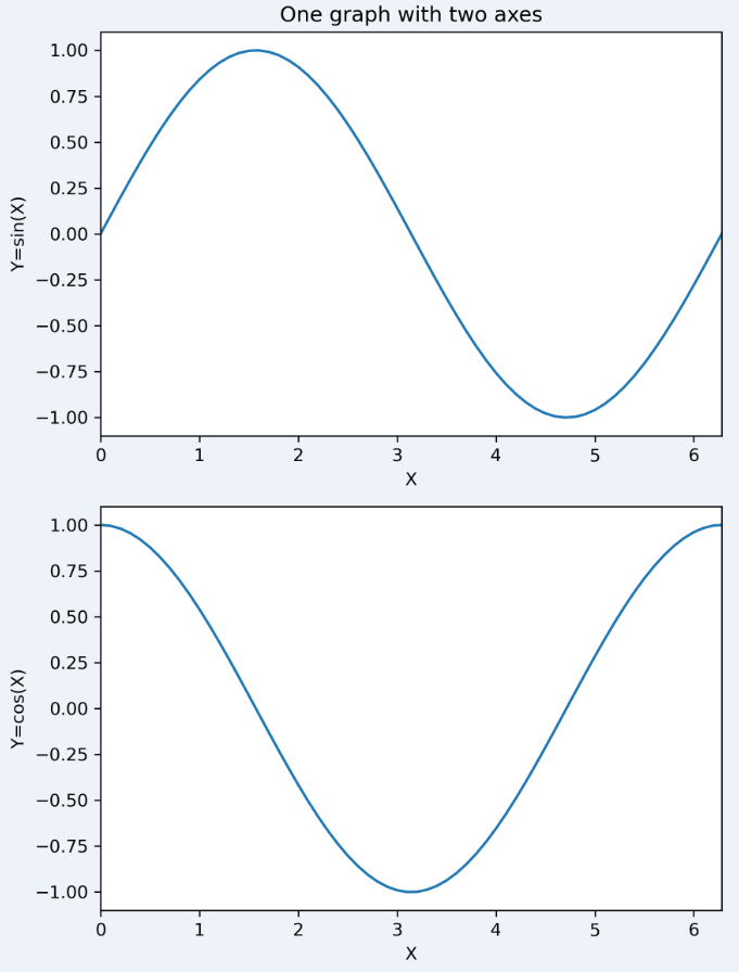
一つの図に二つの座標を作る

import matplotlib.pyplot as plt
import numpy as np

f = plt.figure(figsize=(6,8))
ax1 = f.add_axes([0.15, 0.55, 0.82, 0.4])
ax2 = f.add_axes([0.15, 0.08, 0.82, 0.4])

xMat = np.arange(0, 10, 0.1)
yMat = np.sin(xMat)

ax1.set_title('One graph with two axes')
ax1.plot(xMat, yMat)
ax1.set_xlabel('X')
ax1.set_ylabel('Y=sin(X)')
ax1.set_xlim([0, np.pi*2])

yMat = np.cos(xMat)
ax2.plot(xMat, yMat)
ax2.set_xlabel('X')
ax2.set_ylabel('Y=cos(X)')
ax2.set_xlim([0, np.pi*2])

plt.savefig('F:/Course/python/06/test2.png', dpi=300)

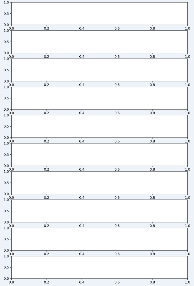
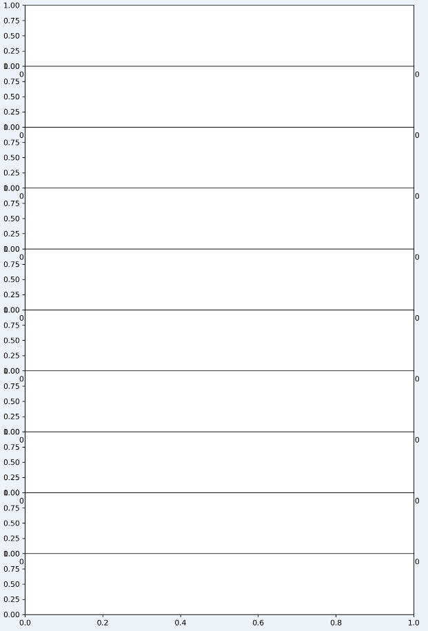
一つの図に十個の座標を作る

たくさんの座標を作るとき、もしこれらの座標は全く同じサイズであれば、ループで作れば便利です。

このような複雑な図を作るとき、まず下図のように図の各部分の位置と大きさを決めるパラメータを設定する。

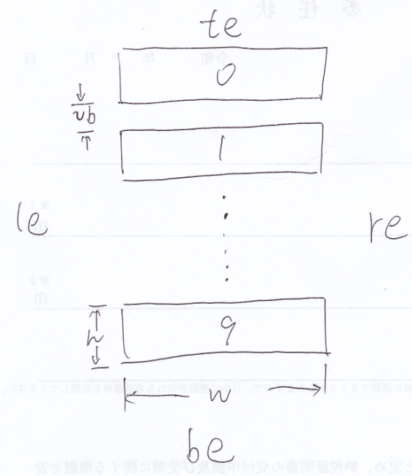
te: top edge
be: bottom edge
le: left edge
re: right edge
w: width
h: height
hb: horizontal blank　（上の図には使われてない）
vb: vertical blank
(これらのパラメータの名前は自分にとって一番分かりやすい名前を付けてください)

これらのパラメータの値を決めれば、図のすべての部分の位置と大きさが決まります。

import matplotlib.pyplot as plt

#図と座標の位置、サイズを決める各値について、
#最初は適当な値に設定して、できた図の形を見ながら、
#最適な値に少しずつ調整する
f = plt.figure(figsize=(8,12))
axNum = 10

be = 0.03
te = 0.02
vb = 0.02
h = (1-be-te-vb*(axNum-1))/axNum

le = 0.06
re = 0.03
w = 1-le-re

axMat = list(range(axNum))
for i in range(axNum):
    axMat[i] = f.add_axes([le, be+(h+vb)*(axNum-1-i), w, h])

plt.savefig('F:/Course/python/06/test3.png', dpi=300)

このようにたくさんのパラメータの設定はちょっとややこしいですが、後ほど図を調整したいときは非常に便利です。例えば、各座標の間の空白は要らない場合は、vb=0に設定すれば、すぐできます。やってみてください。

また、一度作った図は今後同じような図を作るときはコードをコピーするだけですので、非常に便利です。

2. ヒストグラムの作り方

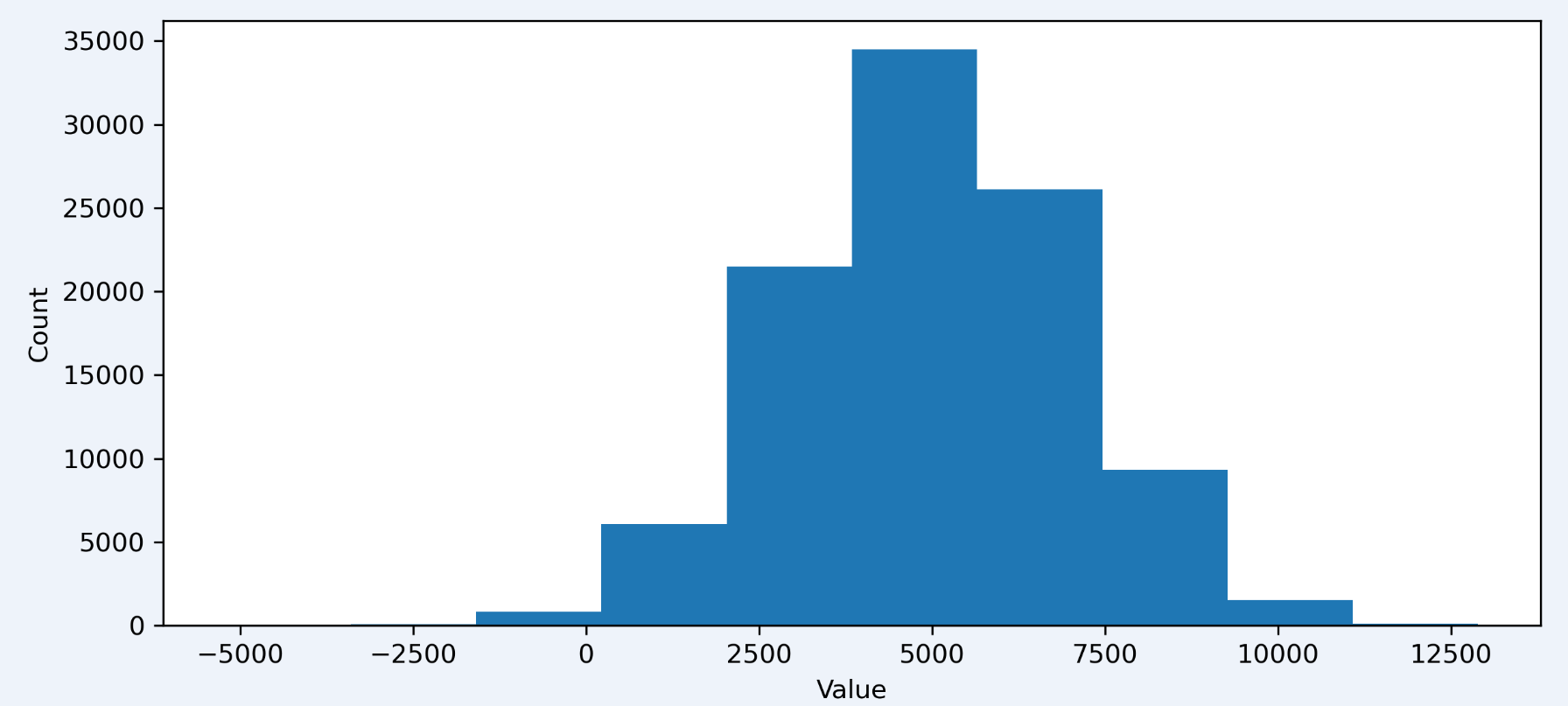
第2回で使われたpython02-2.txtを利用します。このファイルの中にすべての値の分布図を作る。

import matplotlib.pyplot as plt

valMat = []
fid = open('F:/Course/python/python02-2.txt')
while True:
    strLine = fid.readline()
    if len(strLine)==0:
        break
    strMat = strLine.split(',')
    for i in range(10):
        valMat.append(int(strMat[i]))
fid.close()

f = plt.figure(figsize=(9,4))
ax = f.add_axes([0.12, 0.12, 0.82, 0.81])

ax.hist(valMat)

ax.set_xlabel('Value')
ax.set_ylabel('Count')

plt.savefig('F:/Course/python/06/test5.png', dpi=300)

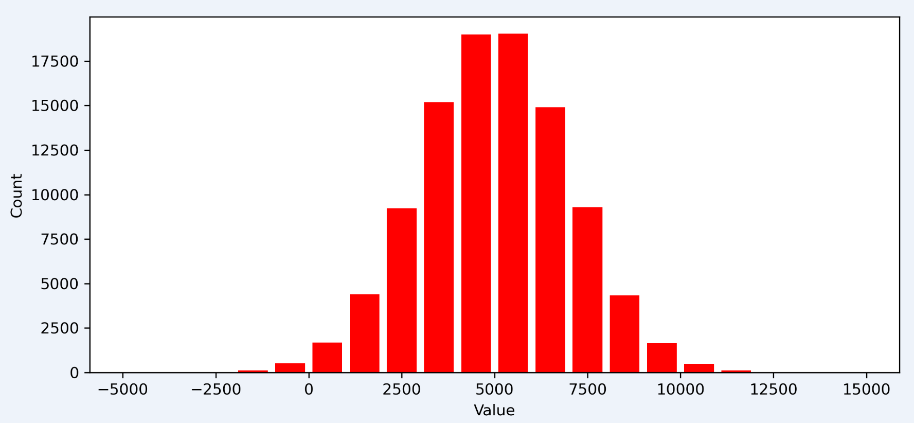
細かく調整する

import matplotlib.pyplot as plt

valMat = []
fid = open('F:/Course/python/python02-2.txt')
while True:
    strLine = fid.readline()
    if len(strLine)==0:
        break
    strMat = strLine.split(',')
    for i in range(10):
        valMat.append(int(strMat[i]))
fid.close()

f = plt.figure(figsize=(9,4))
ax = f.add_axes([0.12, 0.12, 0.82, 0.81])

#-5000から15000までの範囲を20個の棒で示す
ax.hist(valMat, bins=20, range=[-5000, 15000], rwidth=0.8, color='r', edgecolor='none')

ax.set_xlabel('Value')
ax.set_ylabel('Count')

plt.savefig('F:/Course/python/06/test6.png', dpi=300)

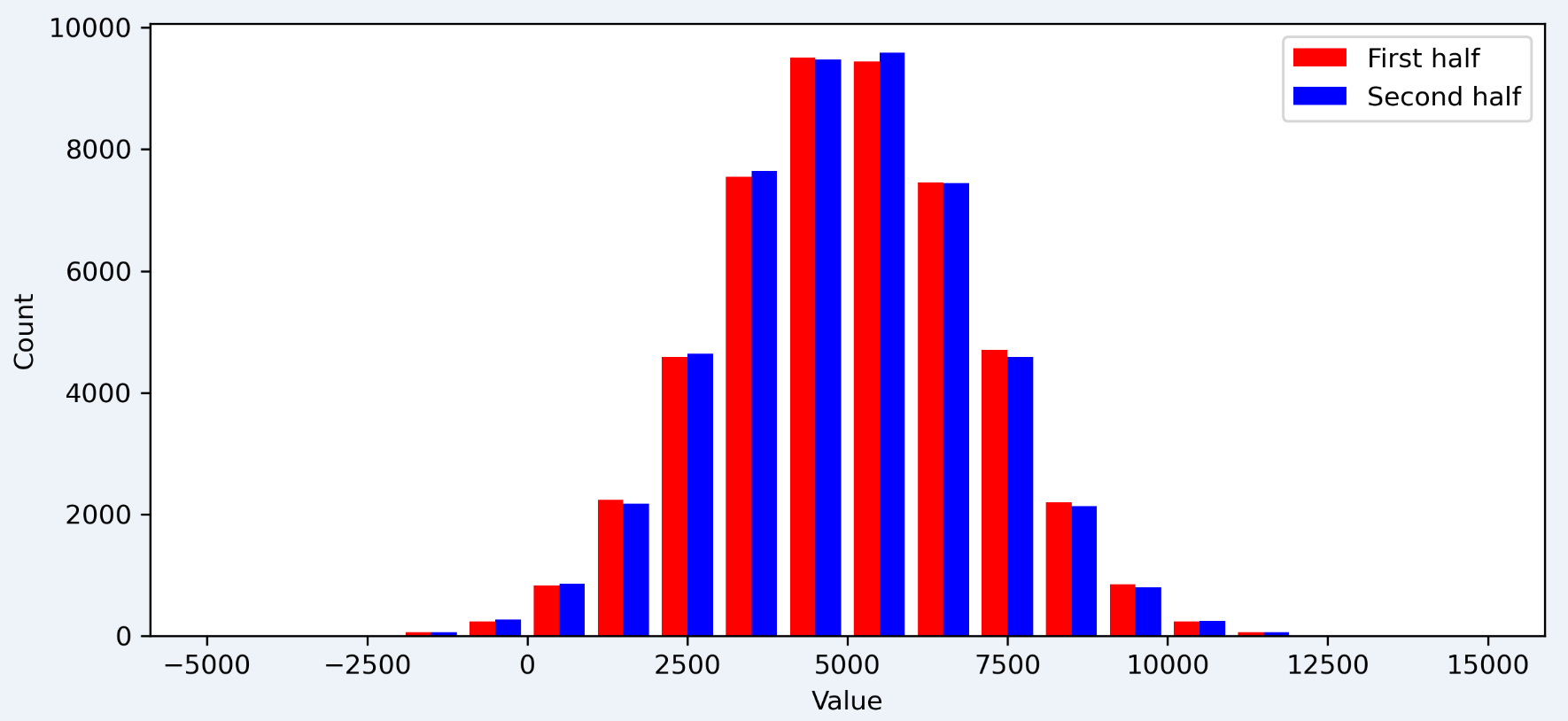
ファイルpython02-2.txtの中の前半と後半の値を分けて分布を作る（二つの分布を一つのグラフにまとめる）

import matplotlib.pyplot as plt

valMat = []
fid = open('F:/Course/python/python02-2.txt')
while True:
    strLine = fid.readline()
    if len(strLine)==0:
        break
    strMat = strLine.split(',')
    for i in range(10):
        valMat.append(int(strMat[i]))
fid.close()

valMat1 = valMat[0:len(valMat)//2]
valMat2 = valMat[len(valMat)//2:]

f = plt.figure(figsize=(9,4))
ax = f.add_axes([0.12, 0.12, 0.82, 0.81])

ax.hist([valMat1, valMat2], bins=20, range=[-5000, 15000], 
        rwidth=0.8, color=['r', 'b'], edgecolor='none', 
        label=['First half', 'Second half'])
ax.legend(loc='upper right')

ax.set_xlabel('Value')
ax.set_ylabel('Count')

plt.savefig('F:/Course/python/06/test7.png', dpi=300)

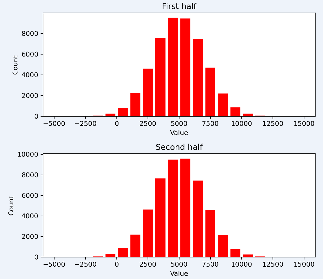
ファイルpython02-2.txtの中の前半と後半の値を分けて、二つの分布を一つ図の二つ座標にプロットする

import matplotlib.pyplot as plt

valMat = []
fid = open('F:/Course/python/python02-2.txt')
while True:
    strLine = fid.readline()
    if len(strLine)==0:
        break
    strMat = strLine.split(',')
    for i in range(10):
        valMat.append(int(strMat[i]))
fid.close()

valMat1 = valMat[0:len(valMat)//2]
valMat2 = valMat[len(valMat)//2:]

#----前述の10個の座標を作るコードを利用する----
f = plt.figure(figsize=(7,6))
axNum = 2

be = 0.1
te = 0.05
vb = 0.13
h = (1-be-te-vb*(axNum-1))/axNum

le = 0.14
re = 0.05
w = 1-le-re

axMat = list(range(axNum))
for i in range(axNum):
    axMat[i] = f.add_axes([le, be+(h+vb)*(axNum-1-i), w, h])
#-------------------------------------

#座標がもっと多い場合は、ループで作ったほうが便利です
axMat[0].hist(valMat1, bins=20, range=[-5000, 15000], rwidth=0.8, 
              color='r', edgecolor='none')
axMat[0].set_xlabel('Value')
axMat[0].set_ylabel('Count')
axMat[0].set_title('First half')

axMat[1].hist(valMat2, bins=20, range=[-5000, 15000], rwidth=0.8, 
              color='r', edgecolor='none')
axMat[1].set_xlabel('Value')
axMat[1].set_ylabel('Count')
axMat[1].set_title('Second half')

plt.savefig('F:/Course/python/06/test8.png', dpi=300)

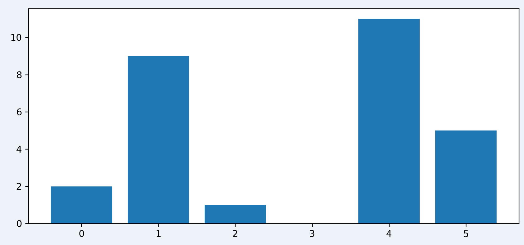
3．棒グラフ

ヒストグラムと似ってますが、扱うデータは違います。以下の例と前述の例と比較してください。

import matplotlib.pyplot as plt

disMat = [2, 9, 1, 0, 11, 5]

f = plt.figure(figsize=(9,4))
ax = f.add_axes([0.12, 0.12, 0.82, 0.81])

ax.bar(range(len(disMat)), disMat, width=0.8, align='center')

plt.savefig('F:/Course/python/06/test9.png', dpi=300)

問題

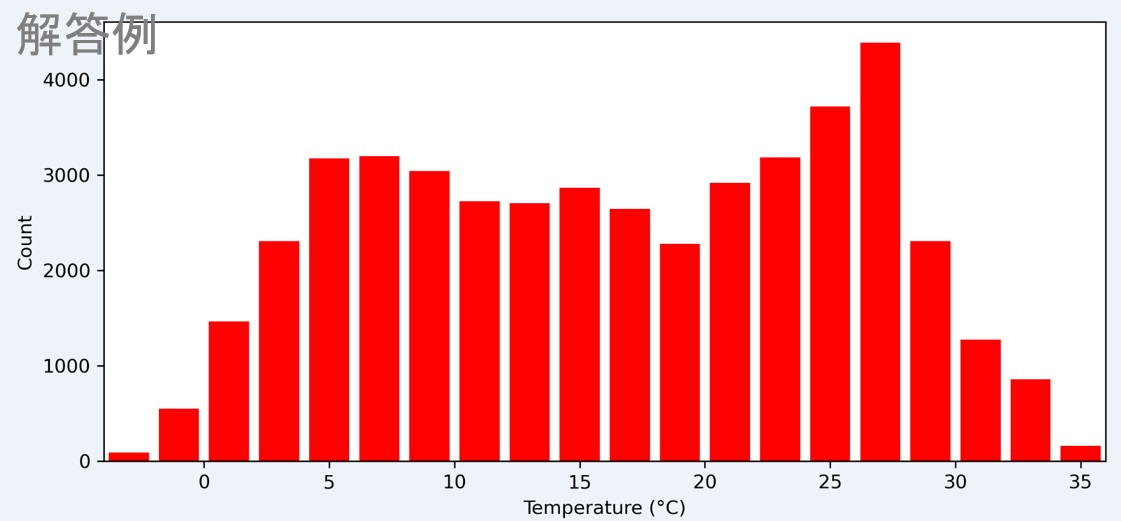
[データ]　前回と同じ岐阜市一年間の温度データを使用する

1．一年間すべての温度の分布図を作る

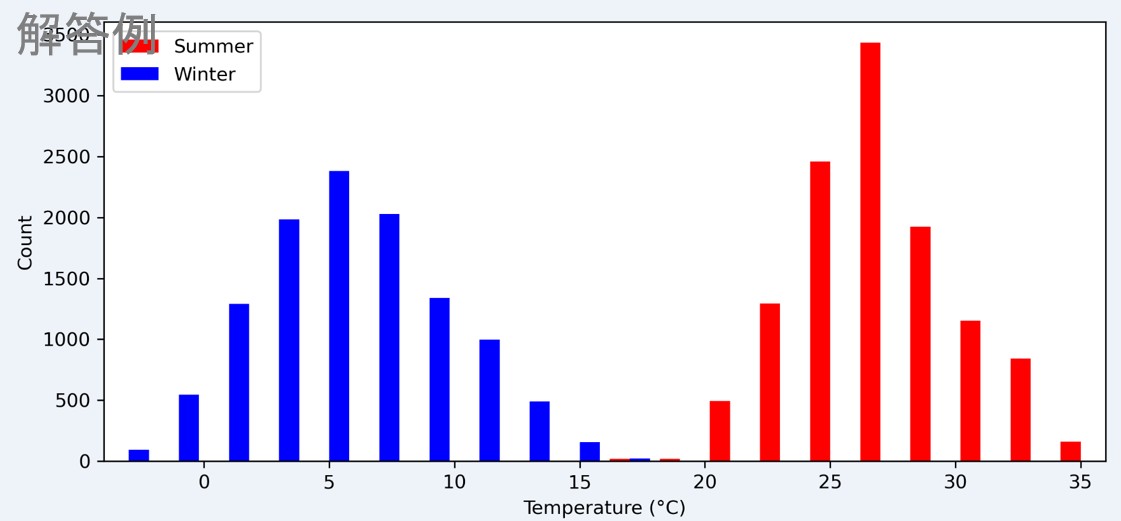
2．7月～9月、12月～2月それぞれ3か月間の温度の分布を一つグラフにまとめて表示する。

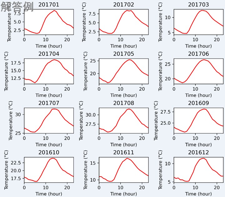
3．各月の温度データにおいて、以下の各時間帯の平均温度を求めて、各月の変化を一つグラフの12個座標に下図のように表す。
[00:00~01:00), [01:00~02:00), … , [22:00~23:00), [23:00~24:00)