FFTによる周波数解析（周波数スペクトラム、フィルター）

Last updated: 2023/01/10

FFT(Fast Fourier Transform)を用いて周波数解析の基本的な方法を紹介します。

1. データ

2020年冬季観測の一つFALMAデータを使います。この時期のFALMAデータには60Hzの交流電源からのノイズがたくさん記録されてました。このノイズを除去する簡単な周波数解析方法を紹介します。
記録の長さは1秒、サンプリングレートは1MHzです。
以下のリンクでデータをダウンロードしてください：
https://tingwu.info/pylab/data/NATL1608070759.bz2

2. 波形のプロット

まず、このデータをプロットして、どんな波形か見てみます。
以下のコードにdataFileのところに実際のデータ保存先を書いてください。

import bz2
import numpy as np
import matplotlib.pyplot as plt

#ダウンロードしたデータの保存先
dataFile = 'D:\data\NATL1608070759.bz2'

sampRate = 1000000　#サンプリングレート
dataLen = 1000 #データの時間の長さ、ミリ秒

fidFile = bz2.BZ2File(dataFile)
dataMat = np.frombuffer(fidFile.read(), np.int16)
fidFile.close()

# Make a figure
f = plt.figure(figsize=(8,5)) 
ax = f.add_axes([0.11, 0.11, 0.82, 0.82])

tMat = np.linspace(0, dataLen, sampRate)
ax.plot(tMat, dataMat)
ax.set_xlim([0, dataLen])
ax.set_xlabel('Time (ms)')
ax.set_ylabel('E-change (DU)')

plt.show()

import bz2
import numpy as np
import matplotlib.pyplot as plt

#ダウンロードしたデータの保存先
dataFile = 'D:\data\NATL1608070759.bz2'

sampRate = 1000000　#サンプリングレート
dataLen = 1000 #データの時間の長さ、ミリ秒

fidFile = bz2.BZ2File(dataFile)
dataMat = np.frombuffer(fidFile.read(), np.int16)
fidFile.close()

# Make a figure
f = plt.figure(figsize=(8,5)) 
ax = f.add_axes([0.11, 0.11, 0.82, 0.82])

tMat = np.linspace(0, dataLen, sampRate)
ax.plot(tMat, dataMat)
ax.set_xlim([0, dataLen])
ax.set_xlabel('Time (ms)')
ax.set_ylabel('E-change (DU)')

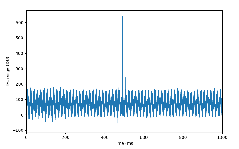
plt.show()

以下のような波形が表示されます。確かに周期的なノイズがあります。

3. 周波数スペクトラム

どんなノイズが存在するか分析するとき、周波数スペクトラムを見れば、ノイズの周波数成分が分かるので、ノイズの成因も推測できます。以下は周波数スペクトラムを作るサンプルコードです。

import bz2
import numpy as np
import matplotlib.pyplot as plt
from scipy.fftpack import fft

dataFile = 'D:\data\NATL1608070759.bz2'

sampRate = 1000000

def getSpectrum(y,Fs):
 	n = len(y) # length of the signal
 	k = np.arange(n)
 	T = n/float(Fs)
 	frq = k/T # two sides frequency range
 	frq = frq[0:n//2] 
 	Y = fft(y) # fft computing and normalization
 	Yhaf = abs(Y[0:n//2])
 	return [frq, Yhaf]

fidFile = bz2.BZ2File(dataFile)
dataMat = np.frombuffer(fidFile.read(), np.int16)
fidFile.close()

f = plt.figure(figsize=(8,5)) 
ax = f.add_axes([0.11, 0.11, 0.82, 0.82])

[freqMat, specMat] = getSpectrum(dataMat, sampRate)
ax.plot(freqMat, specMat, 'r')
ax.set_xlabel('Frequency (Hz)')

plt.show()

import bz2
import numpy as np
import matplotlib.pyplot as plt
from scipy.fftpack import fft

dataFile = 'D:\data\NATL1608070759.bz2'

sampRate = 1000000

def getSpectrum(y,Fs):
 	n = len(y) # length of the signal
 	k = np.arange(n)
 	T = n/float(Fs)
 	frq = k/T # two sides frequency range
 	frq = frq[0:n//2] 
 	Y = fft(y) # fft computing and normalization
 	Yhaf = abs(Y[0:n//2])
 	return [frq, Yhaf]

fidFile = bz2.BZ2File(dataFile)
dataMat = np.frombuffer(fidFile.read(), np.int16)
fidFile.close()

f = plt.figure(figsize=(8,5)) 
ax = f.add_axes([0.11, 0.11, 0.82, 0.82])

[freqMat, specMat] = getSpectrum(dataMat, sampRate)
ax.plot(freqMat, specMat, 'r')
ax.set_xlabel('Frequency (Hz)')

plt.show()

実行すれば、以下の図が表示されます。横軸は周波数(Hz)、縦軸は各周波数成分の大きさを示します。この図を見ると、0Hz(すなわち、直流成分)付近の周波数成分が非常に大きいということが分かります。

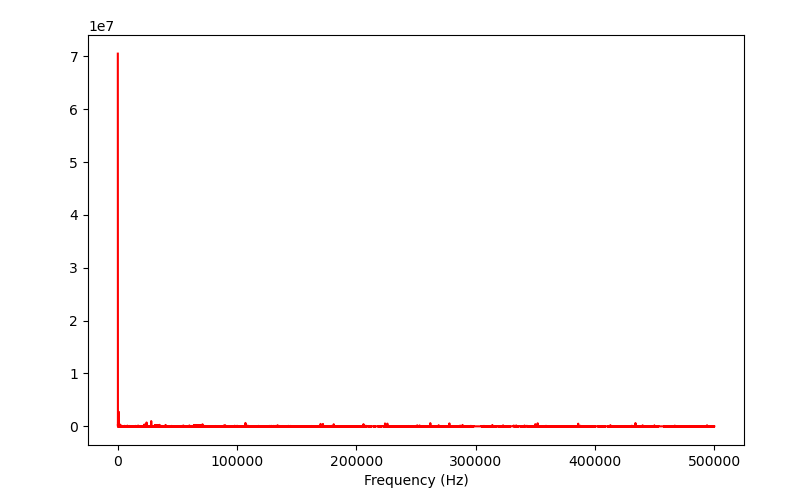
0Hz付近の部分を拡大してみると、

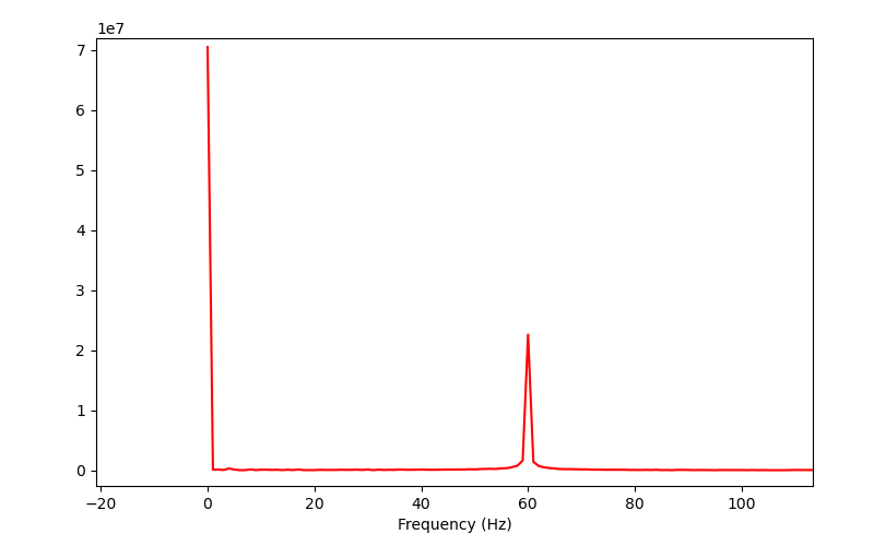
0Hzと60Hzの2つの周波数成分が存在することが分かります。上の波形図をもう一回見ると、波形全体は0より大きいということが分かります。これは0Hz、すなわち直流成分です。そして、周期的な変化(正弦波)をもし数えてみると、1秒間に60個の周期があります。すなわち、これは60Hzの成分です。

4. フィルター

周波数スペクトラムから0Hzと60Hzの成分が非常に大きいということが分かります。これらの成分は明らかに雷信号ではないので、除去したほうがいいです。

以下は100Hz以下の周波数成分を除去する(ハイパスフィルター)コードです。コードの中に、lowFreqとhighfreqは保留する周波数成分の範囲です。すなわち、100Hz以下を除去したいので、残りの成分、100Hzから500kHzまでを保留します。
逆にローパスフィルターを作るとき、例えば、200kHz以上の周波数成分を除去したいなら、lowFreq=0、highFreq=200000に設定すればいいです。

import bz2
import numpy as np
import matplotlib.pyplot as plt
from scipy.fftpack import fft, ifft

dataFile = 'D:\data\NATL1608070759.bz2'

sampRate = 1000000
dataLen = 1000 #ms

#Frequency band to keep
lowFreq = 100 #Hz
highFreq = 500000

waveLen = int(round(sampRate/1000.0*dataLen))
lowIndex = int(round(waveLen/sampRate*lowFreq))
highIndex = int(round(waveLen/sampRate*highFreq))
def filterFun(oriWave):
 	freqMat = fft(oriWave)
 	freqMat[0:lowIndex] = 0
 	freqMat[highIndex+1:waveLen-highIndex] = 0
 	freqMat[waveLen-lowIndex+1:] = 0
 	filterWave = ifft(freqMat)
 	return filterWave.real

fidFile = bz2.BZ2File(dataFile)
dataMat = np.frombuffer(fidFile.read(), np.int16)
fidFile.close()

f = plt.figure(figsize=(8,5)) 
ax = f.add_axes([0.11, 0.11, 0.82, 0.82])

tMat = np.linspace(0, dataLen, sampRate)
filterMat = filterFun(dataMat)
ax.plot(tMat, filterMat)
ax.set_xlim([0, dataLen])
ax.set_xlabel('Time (ms)')
ax.set_ylabel('E-change (DU)')

plt.show()

import bz2
import numpy as np
import matplotlib.pyplot as plt
from scipy.fftpack import fft, ifft

dataFile = 'D:\data\NATL1608070759.bz2'

sampRate = 1000000
dataLen = 1000 #ms

#Frequency band to keep
lowFreq = 100 #Hz
highFreq = 500000

waveLen = int(round(sampRate/1000.0*dataLen))
lowIndex = int(round(waveLen/sampRate*lowFreq))
highIndex = int(round(waveLen/sampRate*highFreq))
def filterFun(oriWave):
 	freqMat = fft(oriWave)
 	freqMat[0:lowIndex] = 0
 	freqMat[highIndex+1:waveLen-highIndex] = 0
 	freqMat[waveLen-lowIndex+1:] = 0
 	filterWave = ifft(freqMat)
 	return filterWave.real

fidFile = bz2.BZ2File(dataFile)
dataMat = np.frombuffer(fidFile.read(), np.int16)
fidFile.close()

f = plt.figure(figsize=(8,5)) 
ax = f.add_axes([0.11, 0.11, 0.82, 0.82])

tMat = np.linspace(0, dataLen, sampRate)
filterMat = filterFun(dataMat)
ax.plot(tMat, filterMat)
ax.set_xlim([0, dataLen])
ax.set_xlabel('Time (ms)')
ax.set_ylabel('E-change (DU)')

plt.show()

実行したら、フィルターをかけられたあとの波形が表示されます。

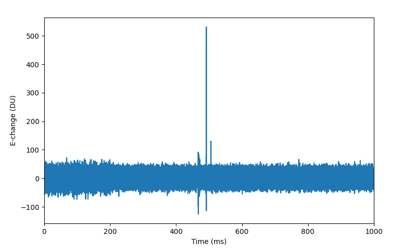
波形全体の基準値は0になりました（直流成分はなくなった）。そして、周期的な変化（60Hzの正弦波）もなくなりました。これらのノイズが除去された後、雷信号の識別も容易になります。

また、いくつか特定の周波数成分を除去したい時は以下のコードを利用してください。delFreqMatは除去する周波数成分の行列です。delWinLenは除去する各周波数成分の幅です。以下のコードでは-5Hzから5Hzまで（負の周波数は意味ないので、実際は0Hzから5Hzまで）、55Hzから65Hzまでの周波数成分を除去します。

import bz2
import numpy as np
import matplotlib.pyplot as plt
from scipy.fftpack import fft, ifft

dataFile = 'D:\data\NATL1608070759.bz2'

sampRate = 1000000
dataLen = 1000 #ms

#Frequency components to get rid of
delFreqMat = [0, 60] #Hz
delWinLen = 5 #Hz

waveLen = int(round(sampRate/1000.0*dataLen))
def filterFun(oriWave):
    freqMat = fft(oriWave)
    for delFreq in delFreqMat:
        lowFreq = delFreq-delWinLen
        highFreq = delFreq+delWinLen
        if lowFreq<0:
            lowFreq = 0
        if highFreq>sampRate/2:
            highFreq = sampRate//2
        lowIndex = int(round(waveLen/sampRate*lowFreq))
        highIndex = int(round(waveLen/sampRate*highFreq))
        freqMat[lowIndex:highIndex] = 0
        freqMat[waveLen-highIndex:waveLen-lowIndex] = 0
        
    filterWave = ifft(freqMat)
    return filterWave.real

fidFile = bz2.BZ2File(dataFile)
dataMat = np.frombuffer(fidFile.read(), np.int16)
fidFile.close()

f = plt.figure(figsize=(8,5)) 
ax = f.add_axes([0.11, 0.11, 0.82, 0.82])

tMat = np.linspace(0, dataLen, sampRate)
filterMat = filterFun(dataMat)
ax.plot(tMat, filterMat)
ax.set_xlim([0, dataLen])
ax.set_xlabel('Time (ms)')
ax.set_ylabel('E-change (DU)')

plt.show()

import bz2
import numpy as np
import matplotlib.pyplot as plt
from scipy.fftpack import fft, ifft

dataFile = 'D:\data\NATL1608070759.bz2'

sampRate = 1000000
dataLen = 1000 #ms

#Frequency components to get rid of
delFreqMat = [0, 60] #Hz
delWinLen = 5 #Hz

waveLen = int(round(sampRate/1000.0*dataLen))
def filterFun(oriWave):
    freqMat = fft(oriWave)
    for delFreq in delFreqMat:
        lowFreq = delFreq-delWinLen
        highFreq = delFreq+delWinLen
        if lowFreq<0:
            lowFreq = 0
        if highFreq>sampRate/2:
            highFreq = sampRate//2
        lowIndex = int(round(waveLen/sampRate*lowFreq))
        highIndex = int(round(waveLen/sampRate*highFreq))
        freqMat[lowIndex:highIndex] = 0
        freqMat[waveLen-highIndex:waveLen-lowIndex] = 0
        
    filterWave = ifft(freqMat)
    return filterWave.real

fidFile = bz2.BZ2File(dataFile)
dataMat = np.frombuffer(fidFile.read(), np.int16)
fidFile.close()

f = plt.figure(figsize=(8,5)) 
ax = f.add_axes([0.11, 0.11, 0.82, 0.82])

tMat = np.linspace(0, dataLen, sampRate)
filterMat = filterFun(dataMat)
ax.plot(tMat, filterMat)
ax.set_xlim([0, dataLen])
ax.set_xlabel('Time (ms)')
ax.set_ylabel('E-change (DU)')

plt.show()

結果の波形は上の波形とほぼ同じです。

Back to Python関連資料